This page has a description of the highlights from the paper, Seligman, D., Shariff, K. "Investigation of a Vorticity-preserving Scheme for the Euler Equations." ApJ, 887, 113, 2019.
The dynamical interaction of vortices in a protoplanetary disk. The color-scale corresponds to the vorticity in the shearing sheet. The simulation was run on 512×512 zones, at a fiducial radius of 1AU, with a sound speed cs= 0.05 and radial and azimuthal extent of.04AU. The Keplerian shear initially dominates the dynamics for the outer two vortices, and the five central vortices merge to form two new ones almost instantaneously. The three long-lived, stable vortices shear past each other for significant evolution, dynamically interacting and exchanging vorticity, before eventually coalescing into a single, much larger whirlpool

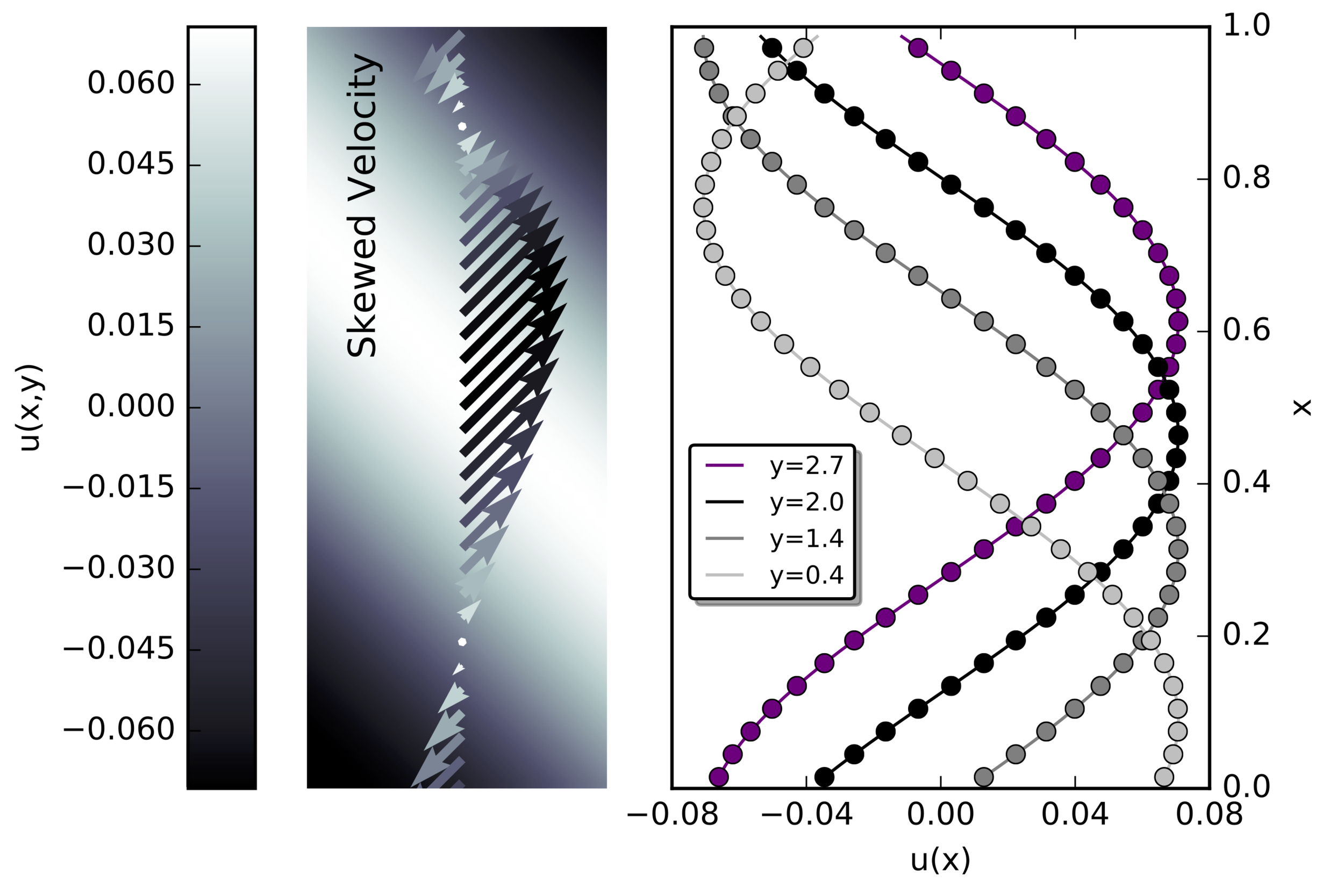
The fidelity with which RBV2 maintains a skewed shear flow on a square grid. The initial conditions for the simulations are shown in the left panel. The color scale in the image corresponds to the x velocity, u(y). The overlaid arrows give a visual representation of the velocity field. In the right panel, the initial analytic solution is shown in the solid lines, and the numerical solution evolved for 60 sound crossing times is shown in x's. The different colors represent different y cross sections of the grid. The corresponding residuals, (u-u_0)/u_0, are shown in grey stars in the middle panel.
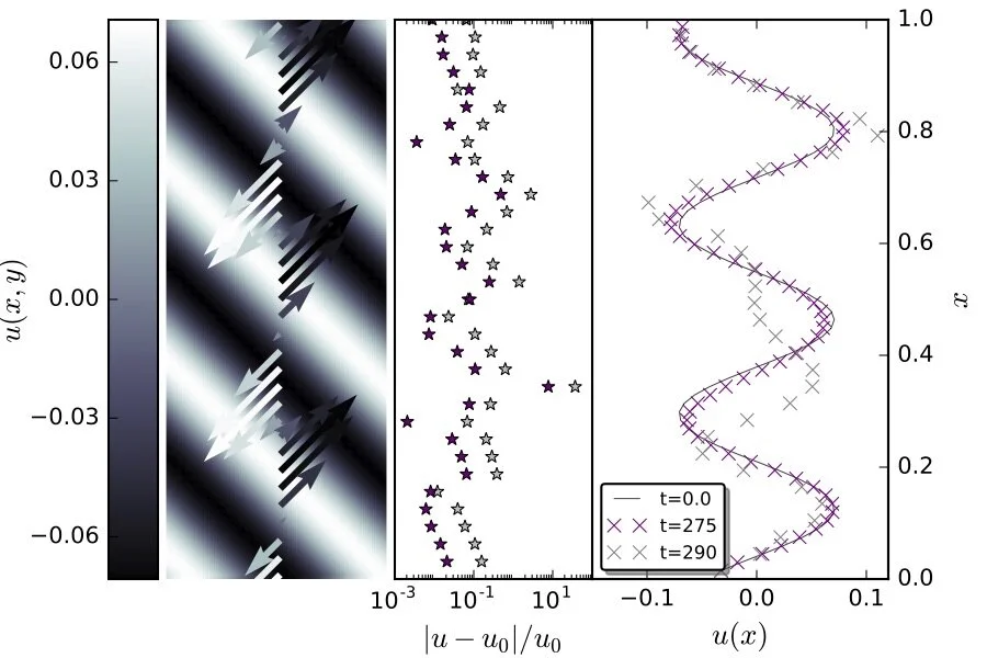
The same skewed shear flow experiment as in Figure 2, with a 4×higher wavenumber. The initial conditions for thesimulations are shown in the left panel. The color scale in the image corresponds to the x-velocity,u(y). The overlaid arrowsgive a visual representation of the velocity field. In the right panel, the initial, analytic solution is shown in the solid lines, and the numerical solution evolved for t∼60 sound crossing times is shown in dots. The purple ×’s show the simulation as the numerical dispersion begins to manifest, and the grey ×’s show the solution as the wave begins to display unsteady behavior. The corresponding residuals, (u−u0)/u0, are shown in grey and purple stars in the middle panel. We initialize the simulation using Equations 18 on a 64×64 zone grid with four times the wavenumber as in Figure 2. The amplitude of the shear flowisA= 0.1, the sound speed is cs= 1 and the domain length is Lx,Ly=√2π. It is evident that the increase in wavenumberincreases the numerical dispersion, as expected
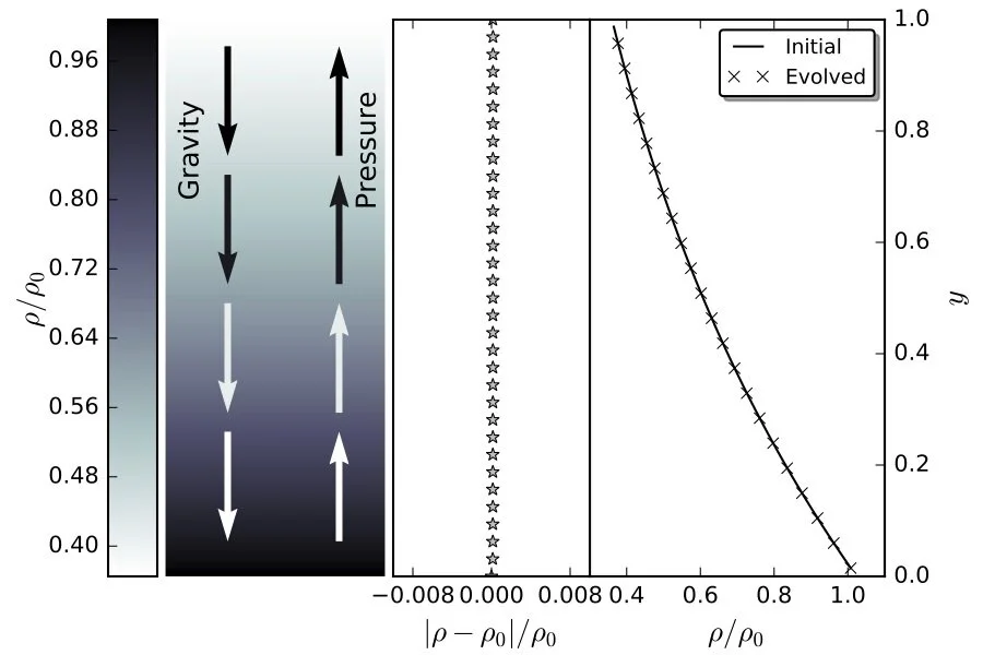
The evolution of a shear flow in the presence of a vertical hydrostatic equilibrium. The initial conditions for the simulation are shown in the left panel. The color scale in the image corresponds to the normalized density,ρ/ρ0. The overlaid arrows give a visual representation of the magnitude and direction of the gravitational body force balanced by the pressure induced by the density gradient. In the right panel, the initial, analytic solution for the density is shown in the solid line, and the numerical solution evolved to 50 sound crossing times is shown in ×’s. The corresponding residuals, (ρ−ρ0)/ρ0, are shown in grey stars in the middle panel. The simulation was run on a 64×64 zone grid, where Lx=Ly= 1,cs= 1,ρ0= 1, and g=−1. It is evident that with the proposed update, the scheme is able to maintain the hydrostatic equilibrium imposed by the external body forces.
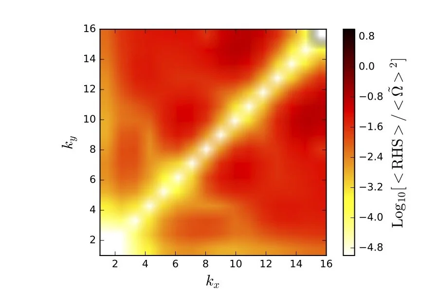
A numerical assessment of vorticity preservation for discrete wavenumber, vortical modes up to the Nyquist frequency. We present the RMS of the residual (RHS) of the vorticity equation normalized by the RMS of the original seeded vorticity fora range of vortical modes. The x and y axes correspond to the wavenumbers kx and ky of the seeded vortical mode. The kx,ky= 0 modes correspond to unskewed shear layers, which have been shown analytically to be vorticity preserving